Confidence Intervals
An alternative way of performing an analysis on data is by means of confidence intervals. While hypothesis testing is a very typical means of analyzing results, confidence intervals can provide more information. They state the possible values that could be the true population parameter of interest. For example, let’s say that you were interested in calculating the mean time of watching YouTube per day. From previous studies, you might believe that the mean is about 1 hour per day. After you collected your sample, your confidence interval states that the possible values range from .5 to 1.5 hours a day. Since 1 hour is within that interval, you have evidence that 1 could be the true mean. However, if you thought that the actual mean was 2 and you had the same interval, then you would have evidence that it is not 2.
It is important to note what we are actually doing when performing this analysis. After we discuss the formula and how to perform a confidence interval, we will discuss the more technical aspects.
Confidence Interval Formula and Usage
Essentially, confidence intervals express the possible values for the true population mean could be for a certain level of error. The equation for calculating a 

Let’s go over the different parts of the formula. 


An important part of this equation is to understand why we divide the error by 2. Let us assume that we want to have an error of .05. When we have confidence intervals, we want to consider both the upper and lower values. Thus, we should split the error in half and put the error at both of the tails. Thus, we would look up a z score or critical value, we would look up the z score value corresponding to .025. Since the normal distribution is symmetric, we only have to look up one of the values since we know that the other value will be the same but just multiplied by -1. When you do examples, you are more than welcome to use your own z table to find the values, but we will use R to get these values. Z tables differ on usage, but essentially, the table should tell you what the critical value is for many common probabilities.
When we perform the confidence interval, we usually believe that the population has a fixed true value of interest. For example, if we were to drop a ball from a tower, we expect gravitational acceleration on earth to be 9.81 meters per second squared. However, we might observe observations or sample means that do not have that value. As long as our confidence interval contains this then, we would have evidence that gravitational acceleration to be 9.80665 with standard deviation of 9.80665. If 9.80665 is not contained in the confidence interval, then our data is incorrect or we do not have evidence that gravitational acceleration is 9.80665. We will go over the intricacies of interpretation in an example.
Example 1
A physicist wants to confirm that the force of gravity behave the same on subatomic particles. Using advanced experimental techniques, she collected the following set of data seen in Table 1 (you can click here for the data as an .RData file). Using the null mean as 9.8067 m/s, do we have evidence that this is true by means of a 95% confidence interval? Explain your result.
|
Table 1 |
|
9.806543 |
|
9.80914 |
|
9.79627 |
|
9.8114 |
|
9.79876 |
|
9.80078 |
|
9.79541 |
|
9.80522 |
|
9.80813 |
|
9.81407 |
Answer 1
To perform a 95% confidence interval, we will use the following formula:


We are 95% confident that the true mean of the population lies between 9.806 and 9.807. Since this does contain 9.8067, we have evidence that the mean is 9.8067. Below is the code to perform this in R.
#example 1

load('Gravity Example.RData')

ls()

xbar<-mean(grav)

sig<-0.001/sqrt(10)

se<-qnorm(.975)*(sig)

xbar+se

xbar-se

#or do this

library('BSDA')

z.test(grav, mu= 9.80665, sigma.x= 0.001)
What does this actually mean?
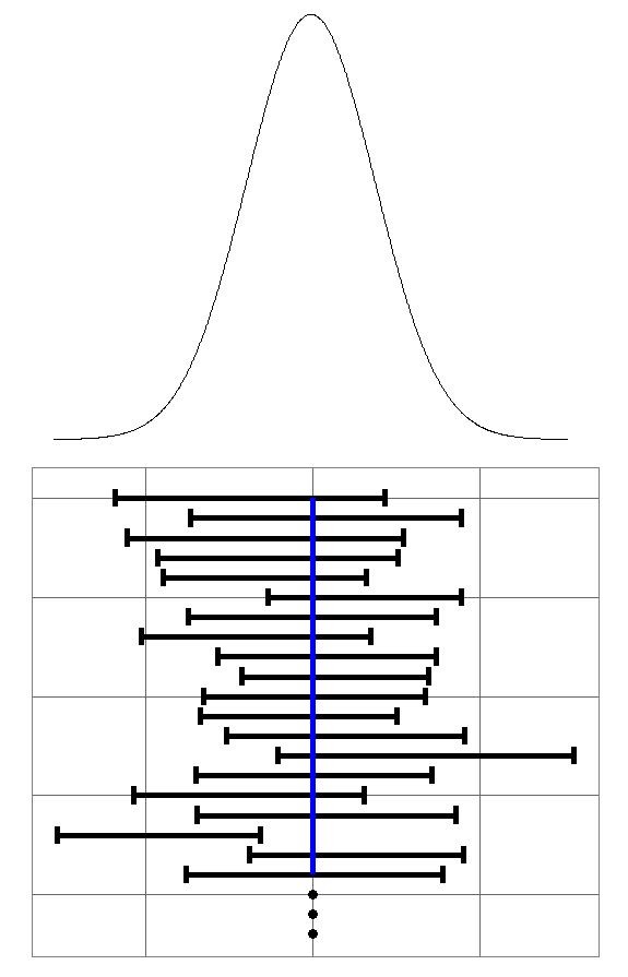
Many people misunderstand what confidence intervals actually state. Remember, the goal of a hypothesis test or confidence intervals are to make inferences about the population from which you sampled from. The sample we received from the population was just one of many. There are many different samples we could have observed from the population of a particular size. Assume that it was possible and easy to pull every single sample from that population. Assume also that you constructed 95% confidence intervals for every sample. We would find that 95% of the confidence intervals would contain the true parameter of interest. This means that 5% will not. The cases are similar for 99% confidence intervals, or any other percentage. We provide an image of this below as Figure 1.

This is important to realize, as performing a confidence interval does not tell us if we observed one that contained the true parameter. Additionally, saying that “We are 95% confident that the true parameter of interest is within our confidence interval” summaries the explanation above succinctly.